Week 1 — What a Pendulum Taught Me About Humanoid Control

Why I’m doing this

I’m working on a research project with JdeRobot around humanoid locomotion: making it easier to give humanoid robots useful movement skills. Before building anything on top of a walking robot, I want to understand how a learned walking policy actually works. A neural network reads some sensor values, outputs some numbers, and a robot with almost 30 joints walks. What happens in between? The physics simulation, the robot state, the observations, the actions and the control.

I’m learning this by rebuilding an existing project piece by piece. My reference is Diego López’s thesis project from Robotics Lab URJC. It runs a walking policy for the Unitree G1 humanoid, trained with mjlab on the MuJoCo physics simulator. My first goal is to make the G1 walk in plain MuJoCo with that trained policy, and to understand every part of it.

This week was about MuJoCo itself. All the code is in the exercises/ folder of the project repository.

Opening up the G1

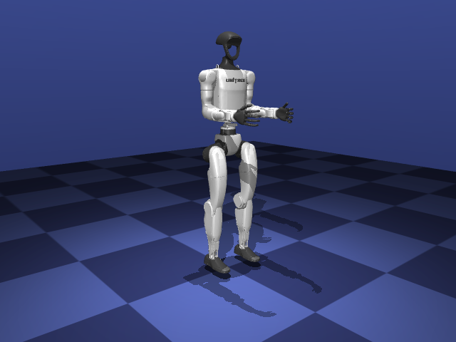
I started by loading the robot and looking at what’s inside. MuJoCo splits a simulation into two objects:

• MjModel holds everything that stays fixed: bodies, joints, masses, sensors, the timestep.
• MjData holds everything that changes: joint positions and velocities, sensor readings, time.

model = mujoco.MjModel.from_xml_path("robot/g1.xml")
data = mujoco.MjData(model)

joint = model.joint(1)                          # look up joints by index or name
print(joint.name, joint.qposadr, joint.dofadr)  # left_hip_pitch_joint [7] [6]

The full inspection script is inspect_model.py.

For the G1:

Quantity	Value	Meaning
nq	36	numbers in qpos (positions)
nv	35	numbers in qvel (velocities)
nu	0	actuators (motors)
joints	30	1 free joint + 29 hinges
sensors	4	gyro, velocimeter, accelerometer, angular momentum

A few of these numbers needed explaining. nq and nv differ because the robot’s base is a free joint that can move and rotate in any direction. Its position takes 7 numbers (x, y, z and a 4-number quaternion), but its velocity only needs 6 (3 linear, 3 angular). So the first hinge joint lives at qpos[7] but at qvel[6], and the reference code has constants for exactly that offset. The quaternion is stored as (w, x, y, z), while SciPy expects (x, y, z, w); mixing them up gives no error, only wrong rotations. And nu = 0 means the file has no motors at all. Without actuators, the robot is a ragdoll.

Free fall and the integrator

The model has no floor, so stepping the simulation makes the robot fall. That makes a nice first test. After time \(t\), the height should be:

\[z(t) = z_0 - \tfrac{1}{2} g t^2\]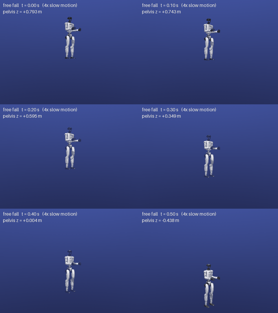

The test itself is only a few lines:

mujoco.mj_resetData(model, data)
z0 = data.qpos[2]                      # pelvis height
while data.time < 0.5:
    mujoco.mj_step(model, data)

t = data.time
z_expected = z0 + 0.5 * model.opt.gravity[2] * t**2   # gravity[2] is -9.81
error = abs(data.qpos[2] - z_expected)

After 0.5 s the formula gives −0.4333 m, and MuJoCo gave −0.4382 m. The simulated robot fell 4.9 mm further than physics says it should.

The difference comes from how MuJoCo moves through time. Its default integrator, semi-implicit Euler, first updates the velocity and then moves the position using that new velocity:

\[v_{n+1} = v_n + g\,\Delta t, \qquad z_{n+1} = z_n + v_{n+1}\,\Delta t\]

Since the robot is speeding up, the end-of-step velocity is the fastest one within that step, so every step moves slightly too far. Summing over all the steps gives the error exactly:

\[z_n - z_0 = g\,\Delta t^2\,(1 + 2 + \dots + n) = \tfrac{1}{2} g t^2 + \tfrac{1}{2} g\,\Delta t\, t\] \[\text{error} = \tfrac{1}{2}\, g\, \Delta t\, t = \tfrac{1}{2} \times 9.81 \times 0.002 \times 0.5 \approx 4.9\ \text{mm}\]

The error is proportional to \(\Delta t\), and halving the timestep did halve it, to 2.45 mm. It’s a small number, but it showed me that the simulator is an approximation with rules I can predict.

One joint at a time: the pendulum

Before giving 29 joints their motors, I wanted to understand a single joint completely. So I wrote a pendulum in MuJoCo’s XML format: one hinge joint, a massless rod of length \(L = 0.5\) m, and a 1 kg ball at the end. The timestep is 0.005 s, the same one the G1 policy uses.

<mujoco>
  <option timestep="0.005"/>
  <worldbody>
    <body name="pole">
      <joint name="hinge" type="hinge" axis="0 1 0"/>
      <geom type="capsule" fromto="0 0 0 0 0 -0.5" size="0.01" density="0"/>  <!-- massless rod -->
      <geom type="sphere" pos="0 0 -0.5" size="0.05" mass="1"/>              <!-- 1 kg ball -->
    </body>
  </worldbody>
  <actuator> <!-- motors go here --> </actuator>
</mujoco>

The model is generated by a small function in pendulum.py, so the later experiments can swap in different actuators.

How long is one swing?

For small swings, a pendulum’s period is:

\[T_0 = 2\pi \sqrt{\frac{L}{g}} = 1.4185\ \text{s}\]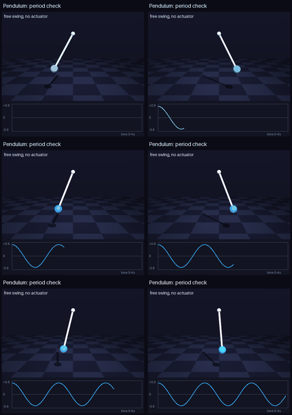

Starting from 0.1 rad, I measured the period by timing when the pendulum crossed zero:

zero_crossings = []
while data.time < 5.0:
    q_prev = data.qpos[0]
    mujoco.mj_step(model, data)
    if q_prev > 0 and data.qpos[0] < 0:     # crossed zero going down: one per swing
        zero_crossings.append(data.time)

measured_period = np.diff(zero_crossings).mean()

It came out at 1.4217 s, about 0.22% longer. That gap can be predicted almost exactly: the ball’s size adds 0.20%, the finite swing adds 0.06%, and timing on a 5 ms grid adds up to ±0.12%. Together that’s 0.14% to 0.38%, and the measurement falls inside.

Where the 0.22% comes from

The ball is not a point. The formula assumes all the mass sits at one point. A real pendulum’s period depends on its rotational inertia \(I\):

\[T = 2\pi\sqrt{\frac{I}{m g L}}, \qquad I = mL^2 + \tfrac{2}{5} m r^2\]

The second term is the sphere’s own inertia (radius \(r = 0.05\) m). Dividing by \(T_0\):

\[\frac{T}{T_0} = \sqrt{1 + \tfrac{2}{5}\left(\tfrac{r}{L}\right)^2} = \sqrt{1.004} \approx 1.0020 \quad\Rightarrow\quad +0.20\%\]

The swing is not infinitely small. The formula uses \(\sin\theta \approx \theta\). The exact period, written as a series, is:

\[T = T_0\left(1 + \frac{\theta_0^2}{16} + \dots\right) \quad\Rightarrow\quad \frac{0.1^2}{16} \approx +0.06\%\]

The timing is quantized. A crossing is only noticed at the end of the step where it happens, so each recorded time can be up to \(\Delta t\) late. Averaging over 3 periods spreads that to at most \(\Delta t / 3T \approx \pm 0.12\%\).

The integrator itself contributes only about \((\omega\Delta t)^2/24 \approx 0.002\%\), which is negligible. All together the prediction is \(0.26\% \pm 0.12\%\), a range of 0.14% to 0.38%, and the measured 0.22% falls inside it.

A PD controller that stops short

Next I gave the pendulum a motor and wrote my own PD controller:

\[\tau = K_P\,(q^* - q) - K_D\,\dot q\]

where \(q^*\) is the target angle. In code, the controller runs before every simulation step and writes the torque into data.ctrl:

def make_pd(kp, kd, target):
    def control(model, data):
        q, q_dot = data.qpos[0], data.qvel[0]
        data.ctrl[0] = kp * (target - q) - kd * q_dot   # torque (N·m) for a <motor>
    return control

The easiest way to picture it is as a spring and a damper:

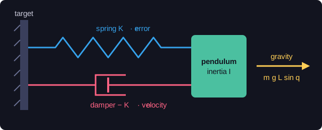
The spring (\(K_P\)) pulls toward the target, harder the further away the pendulum is. The damper (\(K_D\)) resists motion and stops the spring from bouncing forever.

With \(K_P = 20\), \(K_D = 2\) and a target of 0.5 rad, I expected the pendulum to settle at 0.5. It settled at 0.404 rad.

The reason becomes clear once you put the controller into Newton’s second law for rotation:

\[I\,\ddot q = \underbrace{K_P\,(q^* - q) - K_D\,\dot q}_{\text{motor}} \; - \; \underbrace{m g L \sin q}_{\text{gravity}}\]

At rest, both the acceleration and the velocity are zero, which leaves:

\[K_P\,(q^* - q) = m g L \sin q\]

The left side is the spring’s torque and the right side is gravity’s. If the error \(q^* - q\) were zero, the spring would push with zero torque while gravity still pulls down, and the pendulum couldn’t stay there. For the pendulum to hold still, there has to be an error, just enough stretch in the spring to carry the weight. Checking the numbers: \(20 \times 0.096 = 1.93\) N·m, which is gravity’s torque at 0.404 rad. This gap is called steady-state error.

Three ways to close the gap

Rearranging the balance shows the size of the error:

\[q^* - q = \frac{m g L \sin q}{K_P}\]

That points to three fixes.

1. A stiffer spring. The error shrinks as \(1/K_P\). Going from \(K_P = 20\) to 80 to 320 reduced it from 0.096 to 0.028 to 0.007 rad. It never reaches zero, though, and as the next sections show, higher gains bring more overshoot, more torque, and eventually instability.

2. An integral term. Add \(K_I \int (q^* - q)\,dt\) to the controller. As long as any error remains, the integral keeps growing and pushes harder, so the only place the pendulum can rest is zero error. The cost is a slower response and a tendency to overshoot when the motor saturates (called windup). I haven’t tried this one yet.

3. Gravity compensation. If we know the gravity torque, we can simply add it to the motor command:

\[\tau = K_P\,(q^* - q) - K_D\,\dot q + m g L \sin q\]

In code, that’s one extra term:

data.ctrl[0] = kp * (target - q) - kd * q_dot + m * g * L * np.sin(q)

Put that into Newton’s law and gravity cancels out completely:

\[I\,\ddot q = K_P\,(q^* - q) - K_D\,\dot q\]

Now the rest condition is simply \(K_P\,(q^* - q) = 0\), so the error must be zero.

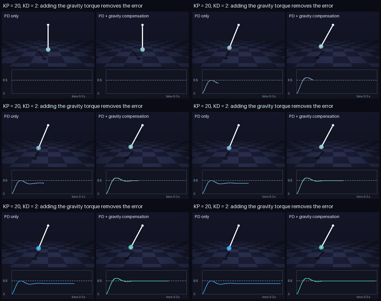
In simulation it settled at exactly 0.5000 rad. The catch is that it needs an accurate model of the robot: its mass, its geometry, where its centre of mass is. On a real humanoid, that model is never perfect.

Predicting the motion

Steady-state error describes where the pendulum ends up. To describe how it gets there, I linearized the system around its resting angle. It then behaves like a mass on a spring with a damper, with total stiffness:

\[k = K_P + m g L \cos q\]

Gravity adds a small extra stiffness of its own, \(m g L \cos q\); that’s where the cosine appears. From \(k\) and \(I\) come the two numbers that describe the whole response:

\[\omega_n = \sqrt{\frac{k}{I}} \qquad\qquad \zeta = \frac{K_D}{2\sqrt{k\, I}}\]

The natural frequency \(\omega_n\) sets how fast it responds. The damping ratio \(\zeta\) sets how much it overshoots: below 1 it overshoots and wobbles, at exactly 1 it reaches the target fastest without overshooting, and above 1 it creeps in slowly. From these, the overshoot and settling time follow:

\[\text{overshoot} = \text{step} \cdot e^{-\pi\zeta/\sqrt{1-\zeta^2}} \qquad\quad t_{\text{settle}} \approx \frac{4}{\zeta\,\omega_n}\]

I implemented these formulas and ran sweeps over the gains to compare them with the simulation. Each formula is a one-line function in pd_experiments.py:

def natural_frequency(k_eff, I):
    return np.sqrt(k_eff / I)

def damping_ratio(kd, k_eff, I):
    return kd / (2 * np.sqrt(k_eff * I))

def predicted_overshoot(zeta, step):
    if zeta < 1:
        return step * np.exp(-np.pi * zeta / np.sqrt(1 - zeta**2))
    return 0.0

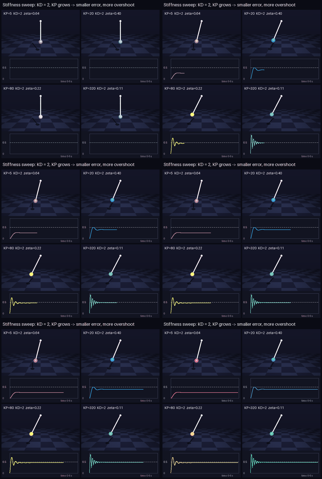
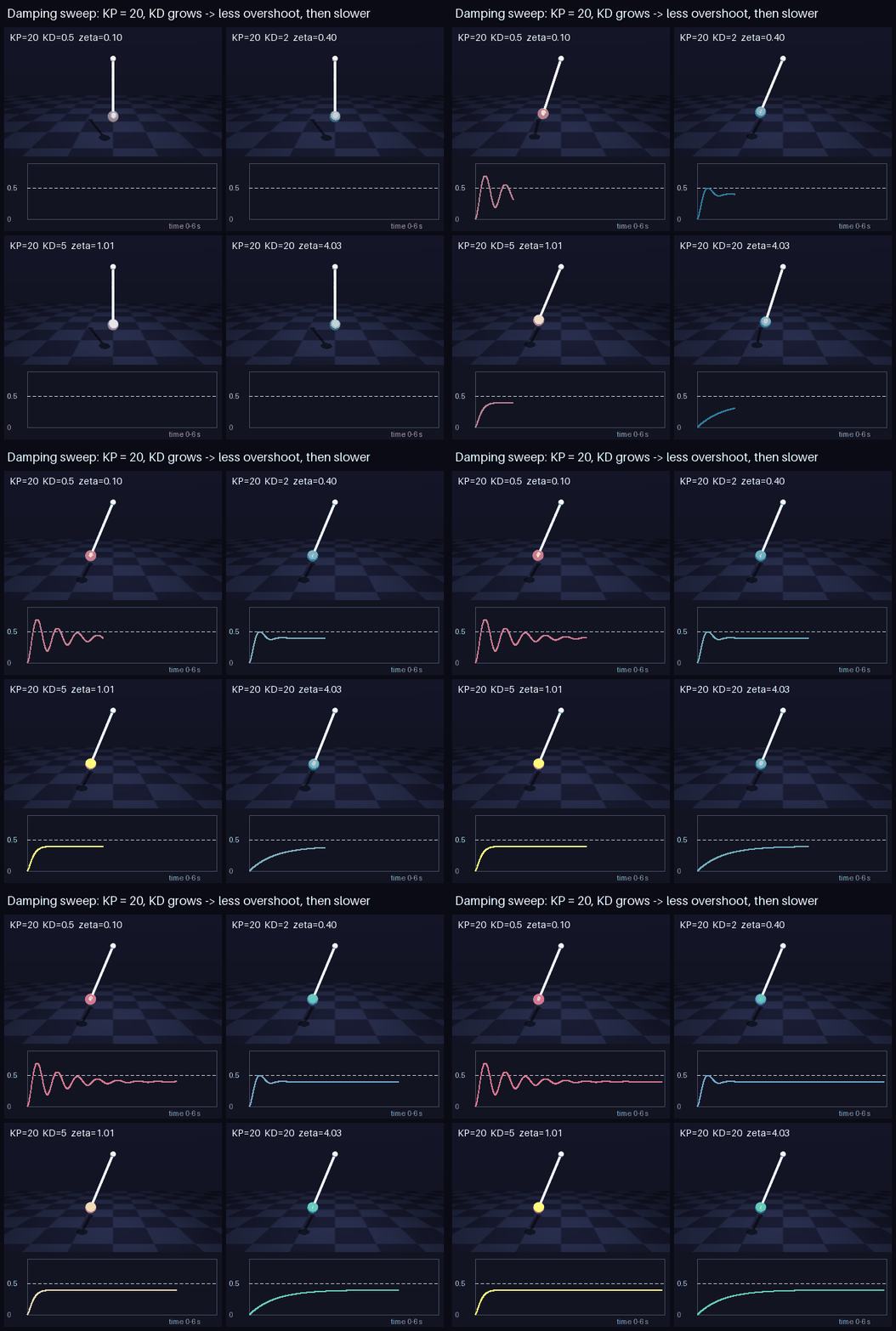
KP	KD	ζ	final angle (sim / theory)	overshoot (sim / theory)
5	2	0.64	0.254 / 0.252	0.018 / 0.019
20	2	0.40	0.404 / 0.402	0.100 / 0.101
80	2	0.22	0.472 / 0.471	0.234 / 0.234
320	2	0.11	0.493 / 0.492	0.348 / 0.347
20	0.5	0.10	0.404 / 0.402	0.295 / 0.292
20	5	1.01	0.404 / 0.402	0.000 / 0.000

Watching a few lines of maths predict the simulation this closely was the best part of the week. The sweeps also made some trade-offs concrete. More \(K_P\) means a smaller error but more overshoot and more torque. More \(K_D\) removes overshoot, but too much makes the response slow again; \(K_D = 20\) took 3 s to settle. Settling speed depends only on \(K_D\) and inertia, because \(\zeta\,\omega_n = K_D / 2I\) and \(K_P\) cancels out, which is why every \(K_D = 2\) run settles in about a second. And critical damping isn’t the fastest option: \(\zeta = 0.8\) settled in 0.38 s with barely any overshoot, quicker than \(\zeta = 1\).

When the simulation breaks

Those formulas assume time flows smoothly, but the simulator moves in steps of \(\Delta t\). If the gains are too high, a single step overcorrects by more than the original error, and the error grows from step to step. For the damping term alone, each step multiplies the velocity by a fixed factor:

\[v_{n+1} = \left(1 - \frac{K_D\,\Delta t}{I}\right) v_n\]

As long as that factor stays between −1 and 1, the motion dies out. Below −1, the velocity flips sign and grows every step. The spring term has a similar limit, and on their own the two give:

\[K_{D,\max} = \frac{2I}{\Delta t} \approx 100 \qquad\quad K_{P,\max} \approx I\left(\frac{2}{\Delta t}\right)^2 \approx 40{,}000\]

These are limits for each term alone, not a combined guarantee. When stiffness and damping act together, a step updates position and velocity jointly, and for this integrator the condition becomes:

\[(\omega_n \Delta t)^2 + \frac{2 K_D\, \Delta t}{I} < 4\]

The individual limits are just the cases where one gain is close to zero. A large \(K_D\) leaves less room for \(K_P\), and the other way around. The simulation matched: \(K_D = 99\) was fine and 101 exploded; \(K_P = 38{,}000\) survived (badly) and 42,000 exploded. Plugging those four runs into the condition gives 3.95, 4.03, 3.87 and 4.26: below 4 for the stable runs and above 4 for the ones that exploded.

MuJoCo’s own actuators

The position actuator

MuJoCo has a built-in position actuator. Every MuJoCo actuator computes its force from one general formula:

\[\text{force} = \text{gain}_0 \cdot \text{ctrl} + \text{bias}_0 + \text{bias}_1\, q + \text{bias}_2\, \dot q\]

Swapping my motor for a position actuator is a one-line change in the XML:

<position joint="hinge" kp="20" kv="2"/>

and the parameters MuJoCo built from it can be printed:

print(model.actuator_gainprm[0, :3])   # [ 20.   0.   0.]
print(model.actuator_biasprm[0, :3])   # [  0. -20.  -2.]

A position actuator sets the gain to \([K_P, 0, 0]\) and the bias to \([0, -K_P, -K_D]\). Substituting gives \(K_P(\text{ctrl} - q) - K_D\,\dot q\): my PD controller, with ctrl as the target angle. Running both versions side by side, the trajectories matched to \(10^{-17}\) rad, which is just floating-point rounding.

Implicit integration

The two versions only behave differently beyond the stability limit. With \(K_D = 102\), just past it, I switched MuJoCo to its implicitfast integrator, which again is one attribute:

<option timestep="0.005" integrator="implicitfast"/>

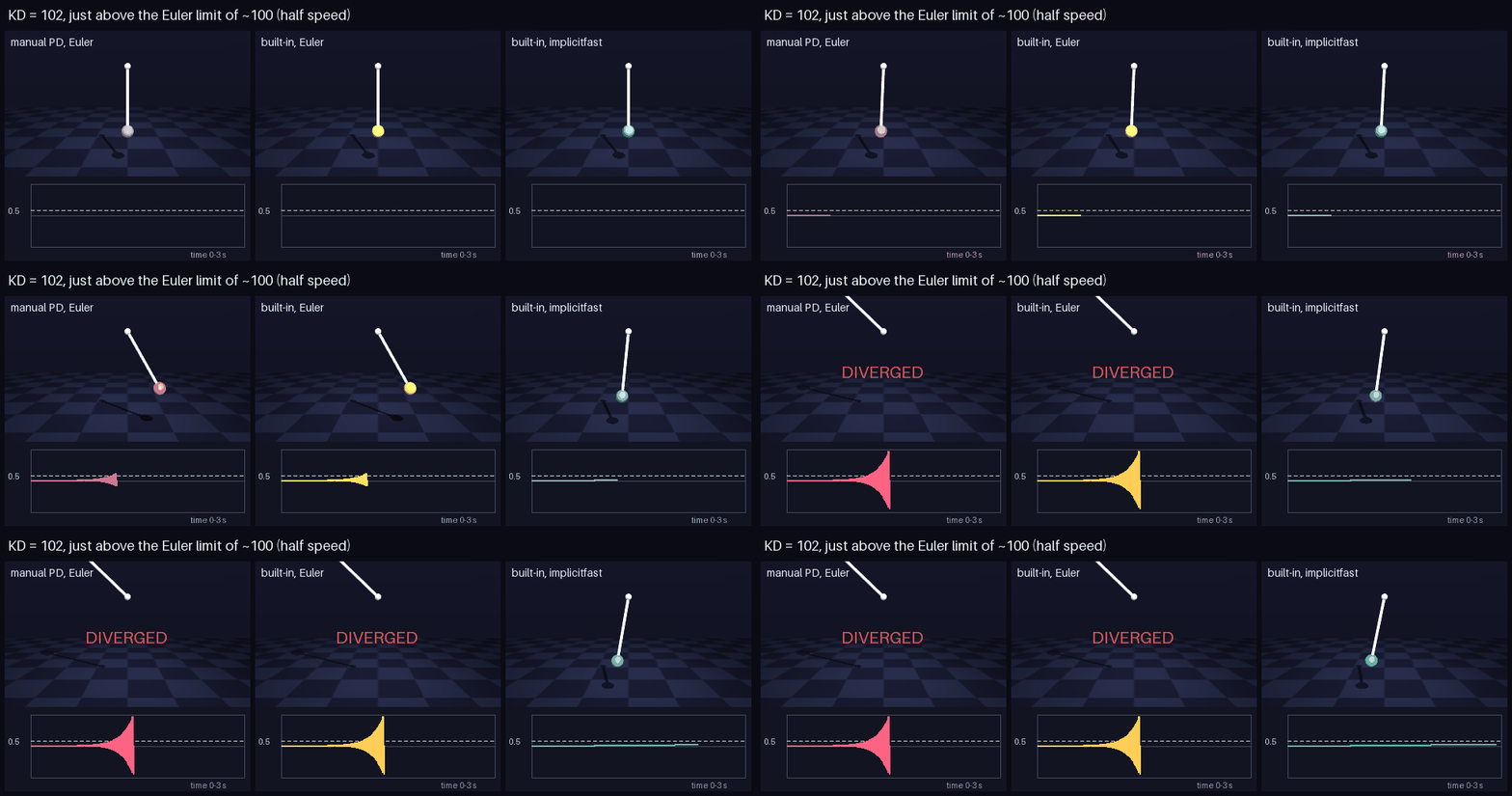
My Python PD still exploded, but the built-in actuator stayed stable. An implicit integrator applies damping using the end-of-step velocity, and that update can never overcorrect, whatever the gain:

\[v_{n+1} = \frac{v_n}{1 + K_D\,\Delta t / I}\]

To do this, MuJoCo needs to know that the force depends on velocity. For the built-in actuator it knows the formula. For my Python PD it only receives a number, so it can’t help. That’s a practical reason to let MuJoCo compute the PD inside its actuators, and a reminder to use the same integrator as in training.

Torque limits

Real motors have a maximum torque. In MuJoCo that’s two attributes on the actuator:

<position joint="hinge" kp="20" kv="2" forcelimited="true" forcerange="-1 1"/>

I limited the actuator to 1 N·m, although holding the pendulum near the target needs 1.93 N·m. I expected it to settle at a lower angle. Instead, it kept swinging between 0 and 0.414 rad and never stopped.

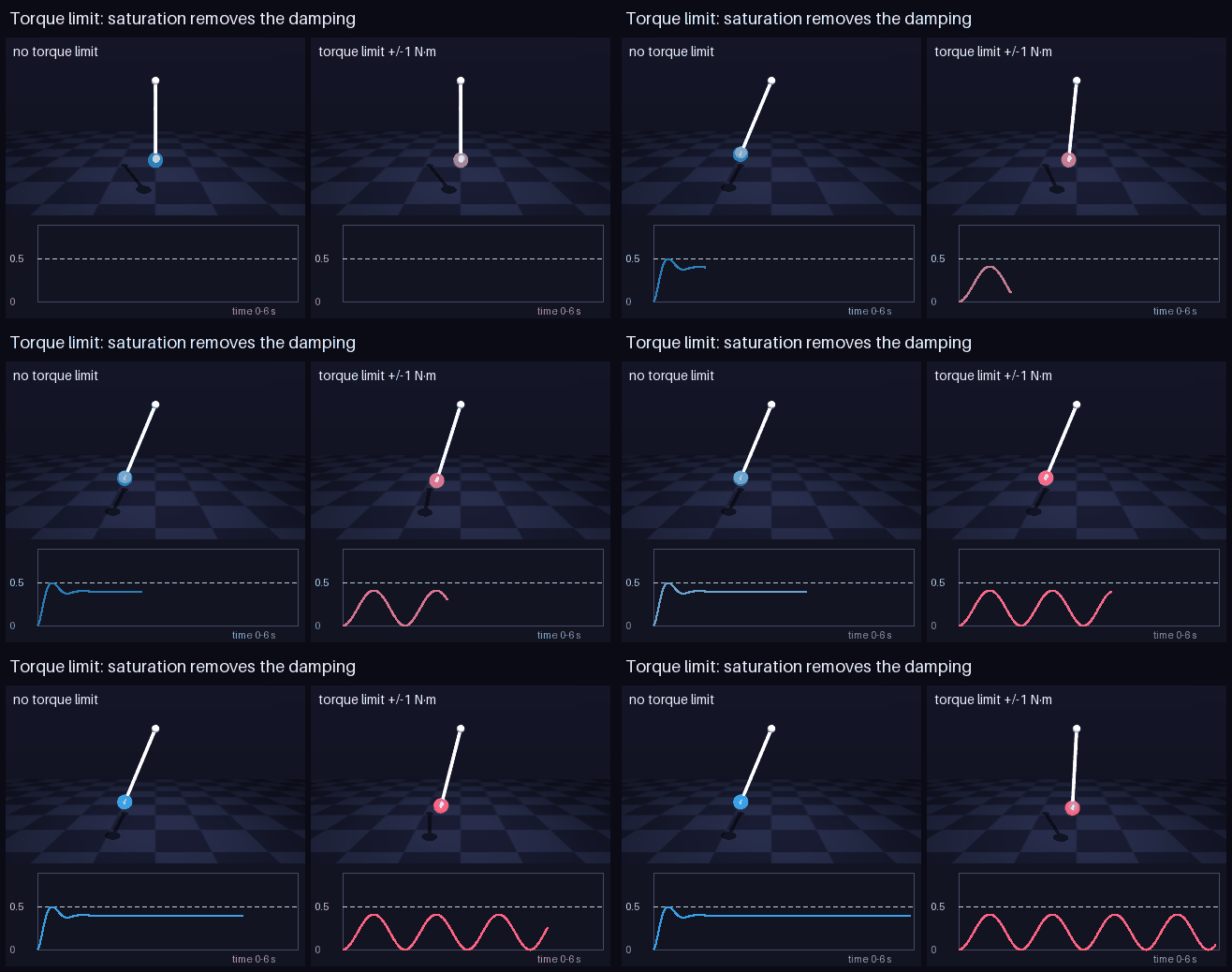
The PD controller asks for more than 1 N·m the whole time, so the motor delivers a constant 1 N·m. A constant torque doesn’t depend on velocity, so the damping term gets clamped away along with everything else. What remains is a pendulum with gravity, a constant push and no damping, oscillating around the angle where gravity equals 1 N·m (0.205 rad). This is actuator saturation: when the requested PD torque goes past the motor’s limit, it gets clipped, and for as long as that lasts the controller can’t deliver the damping it was designed for. Here the saturation never ended, so the damping never came back.

Armature

A motor drives its joint through a gearbox and spins much faster than the joint does. Seen from the joint, the rotor’s inertia gets multiplied by the gear ratio squared. MuJoCo calls this armature and simply adds it to the joint’s inertia:

<joint name="hinge" type="hinge" axis="0 1 0" armature="0.1"/>

After mj_forward, data.M[0] (the joint inertia MuJoCo uses) goes from 0.251 to 0.351. All the actuator experiments are in pendulum_pd.py.

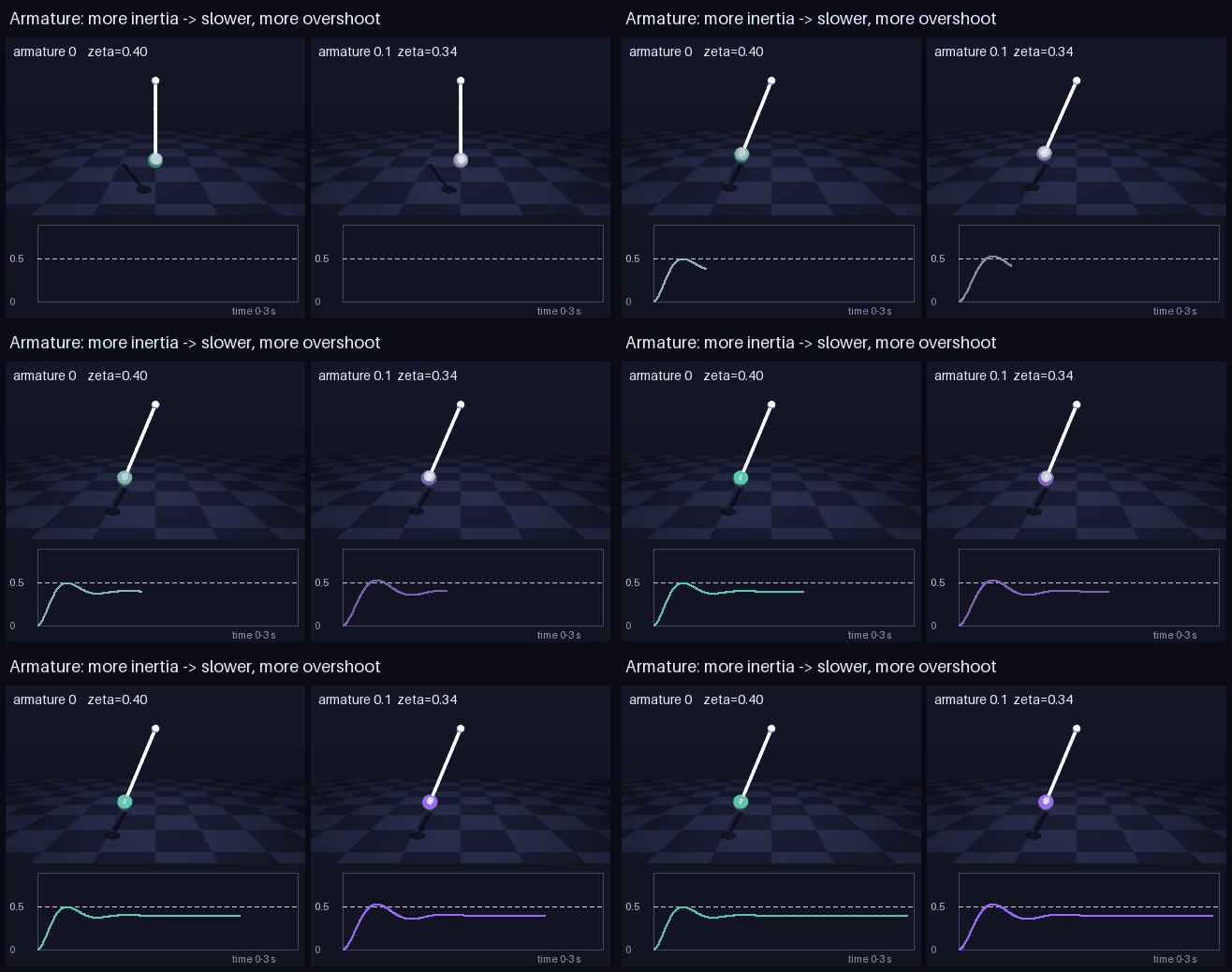
	inertia	ω_n	ζ	overshoot	settle
no armature	0.251	9.88	0.40	0.100	0.84 s
armature 0.1	0.351	8.36	0.34	0.129	1.31 s

More inertia makes the response slower and less damped, just as the formulas predict. The final angle stays the same, because at rest nothing accelerates and inertia plays no part.

From the pendulum to a walking humanoid

All of this matters for the G1 because of where the controller sits. A walking policy could output torques directly, putting control inside the policy. The G1 policy I’m reproducing outputs joint targets instead, and MuJoCo’s position actuators turn them into torques with exactly the PD law above. Control sits outside the policy, in the simulator. Following the usual convention in legged-robot learning, each action is a scaled offset from a default pose:

\[q^* = q_{\text{default}} + \text{scale} \cdot \text{action}, \qquad \tau = K_P\,(q^* - q) - K_D\,\dot q\]

So each pendulum lesson carries over. Because of steady-state error, the policy has learned to aim past the angle it really wants, so that the PD error produces the right torque; change \(K_P\) and every learned action means a different torque. The G1’s gains are computed from each joint’s armature, choosing a 10 Hz natural frequency (\(\omega_n = 2\pi \times 10 \approx 62.8\) rad/s) and a damping ratio of 2, through \(K_P = I\,\omega_n^2\) and \(K_D = 2\zeta I \omega_n\), the same formulas as above. Every joint also has a torque limit. Brief saturation is usually fine, but while a joint is saturated its PD torque is clipped and it can’t guarantee the damping it was tuned for, so persistent saturation can lead to oscillation. And the timestep and integrator have to match training: the policy acts at 50 Hz on top of 200 Hz physics.

How I’m learning

I’m using Claude as a tutor for this project. It suggests the next exercise, explains concepts when I get stuck, and reviews my code, while I write most of it myself. Having something that walks me through a structured sequence and asks “why do you think that happened?” has made a big difference to how quickly I get from confusion to understanding.

Next week

Next week I’ll build the full G1 setup in plain MuJoCo: a floor, 29 position actuators with the right gains, the starting pose, the 99-number observation and the 50 Hz control loop. Then I’ll load the trained policy and, hopefully, watch it walk.